Heat transfer of pipe flows
On the last tab of the heat transfer resistance tool dialog in HTflux you will find a very versatile tool to calculate the heat transfers coefficients (resistances) of pipe flows for gases and liquids.
To get these actual transfer coefficients quite some fluid dynamical calculations are necessary. Fortunately HTflux will do this job for you, apart from the thermal coefficients it will also provide you with many other relevant key figures, e.g. it will calculate the pressure drop for the pipe specified.
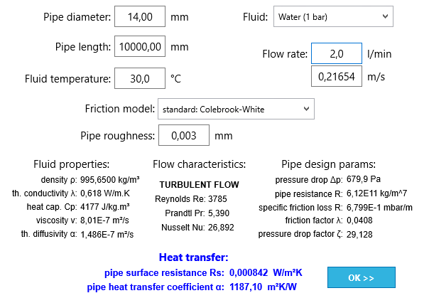
The pipe flow calculation tool
The tool is very powerful if you attempt to calculate the heat-loss (or gain) of pipes containing a flowing medium. This can be relevant for many applications, e.g. heating-pipes, cooling-pipes, ventilation pipes, chimneys, heat-exchanges, boilers, condensers, evaporators, cold-water pipes, hot-water pipes, refrigerator pipes, engine pipes,…
You will only have to specify the desired input parameters. These are:
- Pipe diameter: enter the inner diameter of the pipe.
- Pipe length: enter the relevant length of your pipe.
- Fluid temperature: enter the average fluid temperature here.
- Fluid: here you can pick the type of fluid in your pipe.
Currently the following fluids are available (more can be added on demand):- Water (at 1 bar)
- Air (dry, at 1 atm)
- Refrigerant R134a in liquid phase
- Refrigerant R134a in vapor phase
- Water vapor (steam)
- Ammonia in liquid phase
- Ammonia in vapor phase
- Propane in liquid phase
- Propane in vapor phase
- Isobutane R600a
- Engine oil (clean, unused)
- Flow rate: you can specify the flow-rate in liters per minute here
- Flow-speed: you can specify the average flow-speed in m/s here, the flow rate will be calculated accordindly.
- Friction model: you are able to pick of three different friction models for the calculation:
- Colebrook-White: leave this as default if you are unsure.
- Nikuradse: based on sand-grain roughness
- Smooth pipe model: based on Prandtl calculation
- Pipe roughness: you can provide the absolute roughness of the pipe here, e.g. for PE pipes usually a roughness of 0.003 mm is specified.
After providing the desired parameters HTflux will calculate the surface resistance value of the pipes heat-transfer. By clicking on the “OK” button the value will be assigned for the boundary condition selected. Use this boundary condition along with the correct average temperature in your simulation to calculate the heat transfer of your pipe flow.
Pipe flow and heat transfer physics – brief overview
As HTflux will do the calculation for you, you will not have to dig into fluid dynamics, however the major calculation steps will be outlined in the following paragraphs. The heat transfer from a flowing fluid to the inner surface of the pipe/tube strongly depends on the actual state of the flow. Therefore it is necessary to calculate major characteristic parameters that are used to describe the flow state of the fluid.
After you have selected the type of fluid and its temperature, HTflux determines the relevant properties of your fluid: density, thermal conductivity, heat capacity, kinetic viscosity and the thermal diffusivity. Based on these the so called Prandtl-number is calculated. It is the ratio of the viscosity (momentum diffusivity) and the thermal diffusivity and therefore important for this calculation.
Reynolds number
In a next step the Reynolds-number for the pipe flow will be calculated:
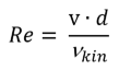
The Reynolds number is an important quantity that allows to predict the flow-state of the fluid. Based on the actual value of the Reynold-number the calculation will continue, either for a laminar (Re<2300) or for a turbulent case (Re>=2300), as these two states of the flow have a considerably different behavior:
Turbulent pipe flow
When the Reynolds-number exceeds a value of 2300 a turbulent flow can be assumed. The turbulence effects lead to a higher rate of “mixing” within the flow and therefore increase the heat transfer rates significantly. The Nusselt-number describing such a flow, can be written as:
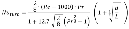
where Pr is the Prandtl-number, Re is the Reynolds-number, λ is the darcy friciton factor of the pipe (see below), d is the inner diameter and L is the length of the pipe.
Laminar pipe flow
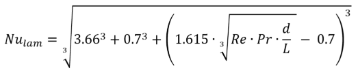
If the Reynolds numbers ranges below the value of 2300 a laminar flow is assumed. In this case a smooth, even flow in the pipe is assumed. The velocity of the flow varies depending on the radius. The highest velocity is reached in the center of the pipe, where the velocity on the surface of the pipe reaches a value of 0. Due to this characteristic distribution the heat transfer to the inner surface of the pipe is significantly lower than in a turbulent flow. For this laminar case the Nusselt-number can be written as:
Friction factors for a pipe flow
As mentioned above you are able to pick among different friction-models. Except for special cases the choice of the model will not have a great impact on the calculation results. If you are unsure we recommend to pick the Colebrook-White model and provide the pipe roughness provided in the specific fact sheet of the pipe or similar documents.
Based on the state of the flow and the model selected, the following equations will be used:
Laminar flow – darcy friction factor
As described earlier, in the case of laminar flow the fluid touching the pipe surface will always “stick” to the pipe surface (v=0). Therefore the friction factor will not depend on the roughness of the pipe in such a case. Consequently the following equation will be used for the darcy friction factor for all laminar flows:

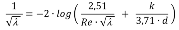
Colebrook-White friction model
For most applications this model will provide the best results. A specific roughness k of the pipe can be provided, however the model will also lead to good results for smooth pipes.
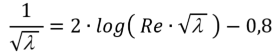
Nikuradse friction model
Based on experiments with sand-grains Nikuradse has developed a friction model, which works best for surfaces with a similar type of “sand-roughness”. The relevant equation for this model is:
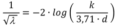
Smooth pipe model
For turbulent flows in ideally smooth pipes the following equation (Karman-Nikurdse/Prandtl) can be used:
Heat transfer coefficient for the pipe flow
After all relevant flow quantities have been calculated, it is easy to finally calculate the heat transfer coefficient of the pipe flow – or its reciprocal surface resistance Rs, as used in HTflux. The Nusselt-number basically contains all relevant information. It only has to be related to the inner diameter of the pipe and the thermal conductivity of the fluid:

Further useful pipe-flow figures: pressure drop, pipe resistance and pressure loss coefficient
Along with the thermal transfer key-figures HTflux provides you also with useful pipe design figures. Using these figures you can easily calculate the pressure drop at given flow rates (or vice versa).
HTflux is using the following equations for this task:
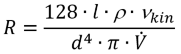
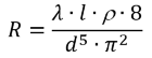
for laminar pipe flows:
Resistance coefficient / hydraulic gradient (R in kg/m7):
Pressure drop (ΔP in Pa):
![]()
Zeta-value (ζ):
![]()
for turbulent pipe flows:
Resistance coefficient / hydraulic gradient (R in kg/m7):
Pressure drop (Δp in Pa):
![]()
Zeta-value (ζ):
![]()
(c) HTflux, Daniel Rüdisser
Note: You are permitted and encouraged to use images from this page or to set a link to this page, provided that authorship is credited to “www.htflux.com”.