Everything you always wanted to know about your heating system…
In the following example two underfloor heating systems are simulated using the dynamic simulation feature of HTflux. Based on these transient simulations we will reveal the differences in the dynamic behavior between these two systems. The precise dynamic behavior is always dependent on the entire setup of the heating system, the floor construction and ambient conditions. Therefore the two examples presented below reflect only two random, but typical, specific configurations.
The two models
The first setup is a so-called dry floor construction, consisting of a dry-screed of a gypsum-fibreboard (25 mm) heated by a special integrated floor-heating system, consisting of aluminum heat plates and PE-heat pipes (14×2 mm) embedded in EPS fixing panels. The second setup reflects a common detail, where the PE-pipes are directly integrated within an anhydrite screed (70 mm). Below the screed, there is an EPS sound insulation board (30 mm).
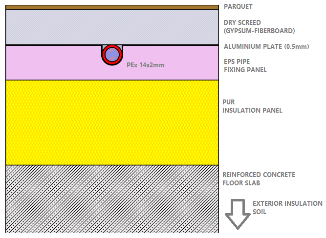
Model A – dry screed & aluminium fins
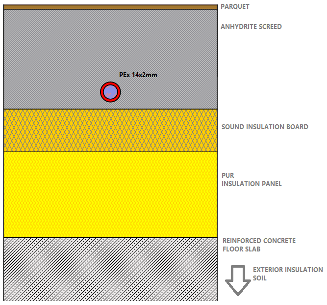
Model B – standard screed
Further both constructions have a parquet layer on top (3mm) and a reinforced concrete slab with exterior insulation below. The pipe spacing distance is assumed to be 15 cm. Due to the symmetric geometry, it is sufficient to simulate only one segment while assuming adiabatic boundary conditions on either side.
The boundary conditions
Consistent with the relevant standard EN ISO 1264 a surface resistance of 0,0926 W/m²K is set for the floor surface (see table on the bottom of heat transfer resistances). The internal temperature is set to 20 °C. On the external side soil contact is assumed (Rse=0 W/m²K, T=10°C). Due to the insulation of the floor slab the exterior side of the model plays a minor role. Of course, the remaining heat loss and its dynamic behavior can easily be studied also, if of any interest.
Specific thermal output of a heating system
Calculating the precise thermal output for the heating system is easy, as you will only have to run a stationary thermal simulation. If you measure the heat-flux to the interior side using the measurement tool and divide it by the temperature difference between the heating medium temperature and the interior temperature, as well as the width of the segment simulated (the pipe-spacing), you will directly get the important gradient of the characteristic curve KH (or equivalent heat transmission coefficient). By multypling this value with the temperature delta, room temperatur minus heating medium temperature, you can easily calculate the specific thermal output q of your heating for any temperatures (the power of your heating per one square-meter).

Heat flux density – underfloor heating, dry system with aluminum plates
E.g. in our first model with the dry screed and the aluminum fins the equivalent heat transmission coefficient can be calculated as KH = Φ / (ΔT·d) = 5,819 / (10·0,15) = 3,88 W/m².K, meaning that for every degree that the heating medium is warmer than the room temperature we will get heating power of 3,88 watts per square-meter surface of the heating system.
The important KH value, that characterizes your heating system, is determined by the thermal conductivities of the layers between the heating medium (pipes, screed, insulation, …) and the floor surface and the actual geometry. Since the thermal simulation performed with HTflux considers all these factors precisely, the calculation results will be more precise than the ones carried out with the methods described in the relevant standard (EN ISO 1264). The calculation guidelines provided there are based on analytic and semiempirical methods, enabling heating designers to get good estimations without thermal simulation. However, as performing such a simulation with HTflux is pretty straight forward, the results will be more accurate and you will get a lot of additional information, we think that this provides an excellent alternative.
Dynamic behavior of a heating-system
Since the calculation of the stationary thermal output is quite easy with HTflux we will proceed to the next level and determine the dynamic behavior of the heating systems, as this will not require a lot of extra effort.
To fully understand and compare the dynamic behavior of the heating systems we define three different cases:
Dynamic analysis I: heat-up/start-up behavior
Of course the warm-up behavior of a heating system does not only depend on the construction of the floor-heating, but also on the heating device, the length of the pipes, thermal masses within the rooms and many other factors. However the thermal mass around the heating pipes usually plays a predominant role. Therefore the best way to study the thermal inertia of the construction is to perform a so-called step-response test. In this test we assume a constant room temperature and an “ideal heater” that is able to provide a constant temperature of heating medium instantly. We first assume the heating pipes in “off” mode, meaning that the water temperature within the pipes will be “floating”, i.e. depending on the surrounding temperatures. From this initial state we will turn on the heating with a so called step function, setting the temperature of the heating medium to a level of 30 °C abruptly at a certain time.
By measuring the following reaction of the system (temperatures and heat-flux) we are able to calculate important time constants, which will allow us to describe the behavior of the entire heating system considering all aspects (like length of pipes, heater output …) later on.

Thermal output during heat-up period – heating medium set to 30°C

Average floor temperature during heat-up period – heating medium set to 30°C
As you can see the construction with the dry screed heats-up significantly faster. To quantitatively describe the thermal mass effect we can use the half-time approach, meaning we can describe the dynamic start-up behavior of the heating system by providing the time it takes until the heating systems reaches half the quantity of its maximum thermal output. This duration is 26 minutes for the “dry screed” system and 104 minutes for the “wet”/standard screed system.
Dynamic analysis II: cooling down behavior
To study the cooling behavior of the underfloor heating we will perform the same step-response test as before. This time will start with an initial temperature of 30°C for the heating medium and abruptly turn off this forced heating. By analyzing the temperatures and heat-flux in this cooling phase we can again gather precious information on the heating system. This information can be used to optimize the control or the design of the heating system.

Thermal output during cool-down period – heating medium set to 30°C

Average floor temperature during cool-down period – heating medium set to 30°C
As you can see the “dry screed” construction cools down significantly faster. The thermal output of the floor drops to half of the maximum amount within 75 minutes, whereas it takes 293 minutes for the “wet screed” construction to reach this level.
Dynamic analysis III: interval behavior
With HTflux you can use any time series to dynamically specify heating medium temperatures. To show a more complex example we have used a 1-hour ON / 1-hour OFF step function as input. Of course the resulting behavior could be deducted analytically from the previously done on- and off-tests, however to study the whole temperature profile it is easier to run a simulation with the according temperature profile. It could be of practical interest to analyze how the underfloor heating-system reacts on such an “interval heating”, as a result either of a poor heating control or a specific heating source running efficiently only at a certain temperature level.

Thermal output during 1h on/off interval mode

Average floor temperatur during 1h on/off interval mode
Comparison “dry screed” vs. “wet screed” heating system
It is important to note that it is not possible to rate the performance of the heating systems solely on these figures. The effect of thermal mass / inertia may be either advantageous or disadvantageous depending on the specific application. E.g. a high thermal mass of an underfloor heating system often causes overheating situations in transitional seasons, when cool nights are followed by a rapid surge in solar gains through windows. Typical heat inputs are displayed in the figure below:
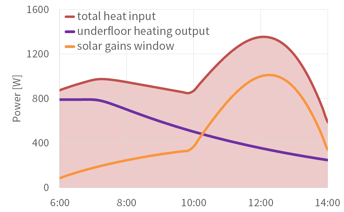
Spring-time overheating situation (south-east oriented room)
On the other hand when, due to technical, economic or ecological reasons, the heating source can only provided power in restricted periods of times, many heating systems rely on high thermal masses. Therefore it is impossible to judge a heating system based on its thermal mass, however it is still important to have a good knowledge of the dynamic behavior to be able to select the system most suitable, as well as to optimize the control of such a system.
(c) HTflux, Daniel Rüdisser
Note: You are permitted and encouraged to use images from this page or to set a link to this page, provided that authorship is credited to “www.htflux.com”.