The following tutorial is very detailed. Getting more and more familiar with HTflux you will be able to go through it very quickly or even to get the job done in an alternative way. Once you have some experience, you will be able to do the simulation below within few minutes.
1. Some important features that you should know
HTflux has a variety of tools that will assist you when drawing or editing objects, that we will introduce briefly:
Navigation controls
It will be helpful to know how you can navigate in HTFlux:
- To zoom in: roll the mouse-wheel forward, while placing the cursor on detail that you want to zoom in on.
- To zoom out: roll the mouse wheel backward.
- To move the view (pan): click your mouse wheel (or middle mouse button). Move your mouse while holding the middle mouse button down.
Hint: if the functions don’t work right away click on the view to make sure that it is activated.
Snap tools
Click on the tools buttons at the bottom right side of the view to activate (blue) or deactivate (grey) the snapping functionalities.
 Grid-snap
objects drawn or edited will be aligned to the grid. To set the dimensions of the grid RIGHT CLICK on the grid-snap button. Point-snap
the cursor will snap to points/vertices of objects already drawn. Line-snap
the cursor will snap to lines of objects already drawn.-
 Angle-snap
the cursor will step to angular lines starting at the reference point. Preset angles are 0°, 30°, 45°, 90°. RIGHT CLICK on the angle-snap button to customize the angles. Turn off the function as soon as you don’t need it anymore, as it can interfere with other snapping tools. - Vertical guideline – X key
when the x-key is pressed the X-coordinate of the current cursor-position will be fixed (“vertical guideline”). This feature is very use full to precisely align objects horizontally. If you press the x-key again the guideline will disappear. - Horizontal guideline – Y key
when the y-key is pressed the Y-coordinate of the current cursor-position will be fixed (“horizontal guideline”). This feature is very use full to precisely align objects vertically. If you press the x-key again the guideline will disappear.
Hint: if keyboard entries don’t work right away. Click into the command line entry field at the bottom of the view, making sure it is activated.
The reference point 
You can use a so called reference point in almost all drawing functions. Use the right mouse button to place the reference point as desired. The reference point is the base point for the angle snap tool, but it also enables you to align point relative to another point. If you type in R 0.5;2.5 in the command line, this will reflect a point being 0,5 units right and 2.5 units above the reference point, that has been set with the right mouse button.
2. The use of project templates
HTflux is a template based Software. This will help you to improve your workflow and save time when working with different types of projects. Just customize the views, grid, units, user-interface and so on in a way that is best for a certain type of project and save your setup using the main menu function Save as template. Later on you can start any new project based on the template that is best suitable for this task. For this tutorial a template called Thermal bridge tutorial is preinstalled. Use the function FILE > NEW and select this template to proceed with the tutorial.
3. Drawing the geometry
In HTflux you have basically two options how you can do a simulation. Either you use the DXF-Import functionality to import a geometry of a CAD software (such as AutoCAD, ArchiCAD, SketchUp…) or you draw the whole geometry in HTflux from scratch. In this tutorial we will use the HTflux drawing functions to model the thermal bridge. Our model will be a simple junction between an exterior wall and an internal floor.
For the dimensions and materials please refer to the following drawing (click to enlarge):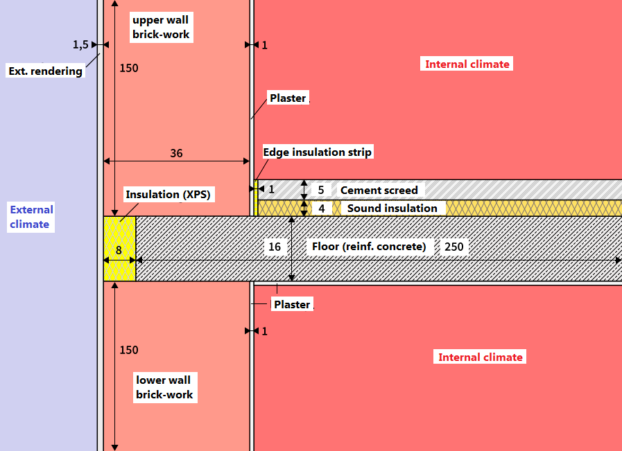
We will use the Rectangle function to draw all the details for this example. Start the function clicking on the Rectangle tool button in the DRAWING menu on top of the screen.

As soon as the function is active a blue text left to the command line will guide you through the function. The text will tell you that state of the current function as well as all possible input options. Now it says “1.point [mouse][x;y][X][Y]”. This means that the function waits for the input of the first corner of the rectangle. This can be done with the mouse [mouse] or by typing in coordinates in the command-line [x;y]. [X][Y] is a hint that you can use the x or y key to align with vertical or horizontal guidelines.
In general it is useful, but not necessary, to type in coordinates for this very first point. This will make sure where the model is placed in terms of coordinates. Type in 0,0 in the command line on the bottom. This will make sure that the first corner of the rectangle is aligned on the coordinate origin. Now the command text tells you that the 2nd corner of the rectangle must be defined, but it also tells you that there are two new input options available:W for width input and H for height input. These functions are essential when drawing construction details, as usually the dimensions of objects are given in the plan.
We will draw the exterior wall of the bottom floor first. Therefore type in W36 (or w 36 in the command line and press the return key, as this wall has a width of 36 centimeters. If you move your mouse now you will see that the rectangle will keep a fixed width now. To set the height type inh150 and confirm with the return key. Move the mouse again the see that now only the orientation of the wall can be set. Move the rectangle to the upper right side a left click with the mouse to finish this rectangle. The first rectangle is ready now. If you have done something wrong you can right click on the object (or in the project manager) to delete the object. While still inside a drawing function you can usually use “U” (for undo) to go back to the previous step.
Now proceed in the same way for the other objects. The following description is just one possible way how you can draw the objects. Once you somewhat familiar with the functions you will use them intuitively and an follow any order you like.
- External insulation strip: move to the top left corner of the just drawn first rectangle. Click on the corner with the left mouse button. Type in w8 to set a width of 8cm and press return. Type in h16 to set the height (the concrete slab will have a height of 16cm). Place the rectangle to the top right direction with the mouse and confirm with the left mouse button.
- Upper exterior wall: Left click on the top-left corner of the insulation strip just drawn. Type in w36 and confirm. Type inh150 an confirm. Place the rectangle to the top right and confirm with the left mouse button.
- External rendering: left click the bottom-left corner of the lower wall and click the left mouse button to set the first corner of the rectangle. Type inw1.5 in the command line and confirm. Now navigate to the top-left corner of the upper wall. Place the mouse cursor there without clicking it. If you are precisely over the point the point snap cursor (diamond) will appear. Now press theY key on the keyboard to have the y-coordinated fixed, this will bring up the horizontal guideline. Now just move the mouse left outside the wall to make sure the external rendering is oriented on the correct side. Left click to finish this rectangle.
- Plaster bottom floor (interior side): move to bottom right corner of lower exterior wall -> left click -> type in width w1 -> move to upper right corner of the lower wall -> fix y-coordinate with Y key -> move mouse rightward outside -> left click to finish.
- Plaster top floor (interior side): move to bottom right corner of upper exterior wall -> left click -> type in width w1 -> move to upper right corner of the upper wall -> fix y-coordinate with Y key, move mouse rightward outside -> left click to finish.
- Concrete slab: move to bottom right corner of insulation strip -> type in width w200 -> navigate to top right corner of insulation strip -> fix y-coordinate with Y key -> move mouse to the right, finish with left click.
- Ceiling plaster: left click bottom right corner of the concrete slab -> type in height: h1 -> move mouse to the right edge of the internal plaster. When line snap is active (cross cursor) -> left click to finish.
Now for the floor layers:
- First the edge insulation strip: left click on bottom right corner of the top floor plaster. Type in width and height: w1 confirm, h9 confirm. Place to the correct side (top and right) and finish with left click.
- Sound insulation: select bottom right corner of the just drawn insulation strip. Type in h4 and confirm. Navigate to right corner of the concrete slab and bring vertical guideline up with x . Place rectangle correct (top side) and confirm with left click.
- Cement screed: left click top left corner of sound insulation. Provide height: h5 confirm. Navigate to top right corner of sound insulation. Type X for vertical guide line. Use mouse to orientate rectangle to the top side. Finish with left mouse button.
- Rectangle for exterior climate: select bottom left corner of the external rendering rectangle for the first corner. Navigate to upper corner of the external rendering and use Y key to get a horizontal guideline. Type in a width for the rectangle. This is actually random, as is it will not affect the simulation. E.g. type in w50 . Place rectangle to the left and finish with left mouse click.
- Rectangle for interior climate: select bottom right corner of lower internal plaster with left mouse click. Navigate to any right corner of the floor construction (e.g. cement screed) and use X key to fix x-coordinate (vertical guideline). Now move to the very top of the wall and navigate to any corner there use Y key to fix the y-coordinate (horizontal guideline). Now the rectangle is fixed, left click to finish it.
IMPORTANT: after drawing the last rectangle the outcome might look unintended. That is because the last rectangle has been drawn on top of the other objects, partly covering them. This “top object cover bottom objects approach” is however useful as you will find out later on. In the next section we will show you how to change the order of objects.
4. Reordering objects
To send the just drawn object (interior climate) to the very back proceed as follows:
Activate the default function Select objects. Either on the left of the top menu or with the small arrow symbol ![]() on the quick tool button below. Now select the object last drawn. You can either do this by clicking on the object in the projectmanager (the last object last drawn will be the top most), or you can click on it in the geometry view. In the geometry view the object will be highlighted in green, and in the project manager the object will get a blue selection box. Now click on the object in the project manager and drag it all the way to the very bottom of the list (holding the mouse button down).
on the quick tool button below. Now select the object last drawn. You can either do this by clicking on the object in the projectmanager (the last object last drawn will be the top most), or you can click on it in the geometry view. In the geometry view the object will be highlighted in green, and in the project manager the object will get a blue selection box. Now click on the object in the project manager and drag it all the way to the very bottom of the list (holding the mouse button down).
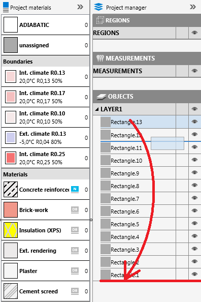
The objects on top of the list will always cover the object further down. This means that now that you have send the internal climate to the bottom of the list, all other objects should be visible again now. Hence you should see you all floor layers again now.
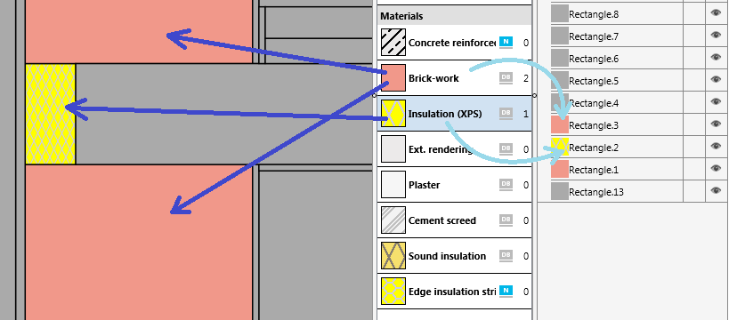
5. Assigning materials
Depending on the task and on your habits there are several ways of how you can assign materials in HTflux:
- You can drag the material from the project material list to the graphical representation of the objects.
- You can drag the materials from the material list to the object list on the right
- You can right click on the objects and open the object properties of the object to change the material.
- You can use the material dropper tool (quick tool bar) for multiple assignments (especially useful on projects with many details)

In our example we will use the first way. If the project material list is not visible click on the Project materials button on the right side of the screen. Now use the left mouse button to select a material and drag it (with the button held down) to the desired objects. Repeat this step until all the objects have their correct materials assigned (see sketch above)
Note: If you double click on a material in the materials list the materials dialog will pop up. Here you can edit all the properties of the material (e.g. the heat conductivity) or you can add new materials from our huge online database. The material dialog will not be explained further in this tutorial.
6. Processing a thermal simulation
We could now continue with adding the psi-measurement tool. However being somewhat impatient, we will run a quick thermal simulation already. That way we can also check if we have done all the material assignments.
To launch the thermal simulation click on the T stable solution button in the main menu (it’s on the START tab):

In HTflux you can draw one or several rectangular regions to define the area where the thermal simulation should take process. To do this use the function REGION on the DRAWING main menu tab.
![]()
In our case we have skipped this step on purpose. When clicking on the simulation button HTflux will now tell you that you haven’t defined any region to be simulated. You will be asked if a region containing all object should be created automatically. Confirm this message with YES.
The simulation dialog coming up now will contain a drop-down list with all the possible regions to be simulated. In our case it will just contain the automatically created region called “total”. In the entry box below you can set the resolution for the simulation. HTflux will guess an appropriate value that you can change accordingly. Higher resolutions will give more precise results. Usually very high resolutions will only be necessary when small metal pieces are involved. The highest resolution that you can process will depend on the amount of physical memory that you have installed and available. HTflux will show you this amount in graphic representation. If you have many programs running at the same time you will see how the memory available will start to increase once you close these programs. The solver algorithm of HTflux is quite fast so the resolution of your simulation will in fact only be limited by the physical memory available. For this reason we highly recommend to run HTflux on 64-bit Windows versions, as the memory available in 32-bit environment is very limited.
Back to our example: accept the resolution suggested by the program and process the simulation by clicking on the blue button “start simulation”.
Within seconds you will see a temperature view of the detail just drawn. You can now use the mouse to navigate through this temperature view just like before (zoom with mouse-wheel and so on). Clicking on the top menu button HEAT FLUX you can change to the heat flux view to actually see the effect of the thermal bridging. Clicking on the button Display settings on the bottom of the screen you will find many options to customize each of the views. You can e.g. change the color palette, change the resolution of the isotherms, and many more. However these options are not a topic of this tutorial.
7. Using the automatic PSI-measurement tool
To continue with the thermal bridging calculation you should select the material view now. Basically you can work in any view, but usually tool function can be applied more easily in geometric views.
Change the top menu bar to the MEASUREMENTS tab and select the automatic PSI function there:
![]()
Just like before the text left to the command line will provide helpful hints when applying the function. In this case it says “Set anchor point of leg A”. With this step you will define the range of the flux measurement as well as the boundary side on which the flux measurement should take place. According to the ISO standard the section has to be further than 1 meter or three times the thickness of the flanking floor away to make sure that the effect of the thermal bridging has vanished there and the isotherms will be parallel again. HTflux has a unique feature that will display the theoretic, 1-dimensional U value of the wall as well as a “measured”, flux base two dimensional U value that will allow you to judge if the criterion just mentioned is met. If you are too close to the thermal bridge, or if you have other disruptions involved the U values will deviate strongly.
Related to our example it is sufficient to place the anchor points of the leg on the internal (or external) boundary of the wall and make sure that they are at least one meter away from the floor junction area.
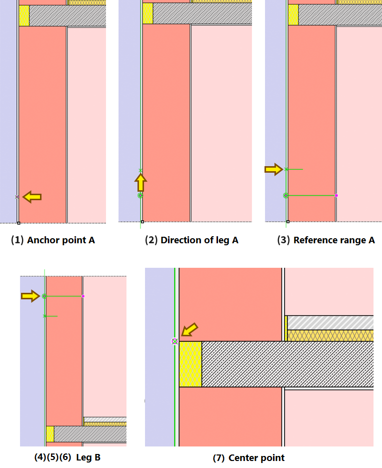
Let’s return to the PSI function, step by step:
- Anchor point A: place the anchor point with the mouse (or by text input). E.g. set it on the internal side close to the bottom of the wall (or on the edge).
- Direction of leg A: now you have to define the direction of the leg for the PSI calculation. In this example the direction will be strictly vertical for both legs. So just click on the same boundary somewhere above the point just set to get a strictly vertical line.
- Reference range of leg A: to calculate the additional 2d U-value the input of length for this reference section is necessary. You can either set this length with the mouse or you can type in 25 to precisely define this length. This means that base on a 25cm height section just above the first anchor point HTflux will calculate a 2d U-value base on the actually measured heat-flux.
- Anchor point B: now place the anchor point for the upper wall. You can set it right on the top edge where the internal climate meets the wall or somewhat further below.
- Direction of leg B: set the direction downward in precisely vertical line.
- Reference range of leg B: type in 25 again or set it with the mouse.
- Center point for calculation: this step is only necessary when calculation PSI values with parallel legs, like in our case. If you are doing the calculation on cases with non-parallel legs (like corners), the intersection of the two legs will automatically be defined as point of reference. Here it is necessary to define a point where the leg with the U-value A switches to the leg with the U-value B. You will have to set this point according to your building energy calculation model. The actual position depends on local standards or processes defined by authorities. Often the upper edge of the floor slab is defined as this point. Therefore we use this point in the tutorial. Anyway in this example, where the upper wall has the same U value as the lower wall, the position of this point is not relevant for the result, as the calculation will always give the same values.
Hint: if you have done an entry wrongly you can go back (undo) using the U key
The setup of the PSI-measurement tool is no complete. To process the calculation you will simply have to rerun the simulation. To do this click on the T-Stable Solution button in the START menu again.
8. PSI Measurement Tool: display options and dialog
Now after processing the simulation a so called “tag” which will give you the result of the calculation will show up. Every measurement function will bring up one or more of these tags. The tags offer a number of options to optimize or customize the result display:
- You can move the tag when clicking on it and holding the mouse button down.
- Using the tiny + and – button on top you can increase or decrease the size of the tag
- With the tiny down arrow button you can display details for the measurement
- Clicking on the tiny X button you can hide the tag. To bring it up again double click on the round marker
- Double click inside the tag area to open the specific tool dialog, where you can further customize the tool.
If you cannot see any tags or markers, check if the result display is turned on. To do this make sure that the tag button ![]() in the quick tool menu at the bottom is activated (blue).
in the quick tool menu at the bottom is activated (blue).
To better explain the functionality and option of the PSI-tool click on the small details button (arrow down):

The tag will enlarge and give you additional parameters:
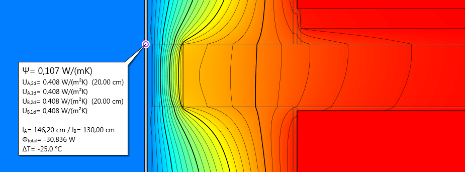
- Ua,2d: the U-value of leg A (here it’s the lower exterior wall) calculated based on the simulated heat flux in the previously defined reference range having a height of 25cm
- Ua,1d: der U-value of leg A, calculated based on the resistivities and thicknesses of the material layers and heat film coefficients. (see further below)
- Ub,1d, Ub,2d: like above, but for leg B (upper wall)
- lA,lB: the lengths used in the calculation. Depending on the resolution of the simulation these values can be slightly adjusted to get higher precision. The lengths reflect the actually relevant parameters for the caluclation.
- Φtotal: total heat flux through leg A and B.
- ΔT: the relevant temperature difference for the calculation.
The calculation of the 2d values along with the 1d U values allow you to judge the quality of the simulation very easily. If the variation is within very few per cents the quality of the simulation is sufficient. If the variation is higher you are either too close to the thermal bridging spot or there is another disruption within the area where the heat flux is measured. One special case that should be noticed is when you have a periodic construction structure within one or both legs (like beams running through the wall). In this case you should define the range of the 2d reference area as the periodicity length of these structure and use only the 2d values for the calculation. To do this double-click on the tag and select the 2d values in the dialog.
The PSI-dialog also contains further options (like dealing with temperature factors) as well as another mode to calculate the PSI-value. These options are not part of this simple tutorial.
Using the detail parameters displayed above one can redo the PSI calculation that HTflux does internally. The calculation is based on the following formula:
When redoing the calculation “by hand” there might be a small deviation, as HTflux is internally taking more than the displayed digits into account.
Another add-on feature of the PSI tool is the possibility to also display the U value and layer configuration for the two legs. To show that extra information double-click on the round markers representing the legs of the PSI-calculation.
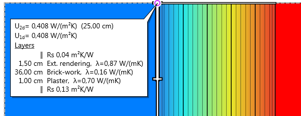
When they open click on the tiny “detail” button again to also display the layers of the wall. If you double click you have a variety of options to further customize the display.
8 Alternate method to determine the Ψ-value using the total heat flux tool
[optional]
Just for completeness we will show you how you would do this calculation with the heat flux measurement tool. This would be the “Therm like” way of doing it. Anyway, using the automatic PSI tool will help you to save time and give you extra information, so there is usually no reason to do the calculation “by hand”. We will do this extra step to demonstrate the use of the Heat-flux measurement tool as well as to better explain the math and defintion of the PSI-value (aka. linear thermal transmittance coefficient).
Since we will have to determine the total heat flux for the „manual“ calculation you will have to add heat flux measurment tool to your project. This is simply done, by pressing then Heat flux button (in the Measurements menu):
![]()
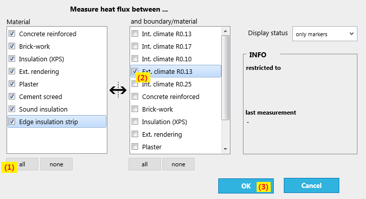
In the project manager on the right side of the project you will find a new entry called Heat flux.1 listed in the section Measurements. The measurement itself will be done inside a selected region on any appropriate boundary between a boundary condition and material or between different materials. In this case, as in most cases we are interested in the total flux of a boundary condition. To define this please double-click on the newly added Heat flux.1 entry to open the settings dialog of this tool. To define the boundary flux click on the all button (1) for the right material list and select external climate (2) on the right material list. Now HTflux will measure the flux wherever the boundary condition external climate touches any material. You could as well select all the internal climates instead of the external climate. Due to energy conservation the flux has to be the same, only the sign of the flux will be different. Now you can already close (3) the dialog.
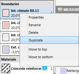
As mentioned the second thing to do is to define a region in which the measurement should take place. We could define any region using the region tool to draw one or more regions. Since we do not want to limit the flux measurement to a certain reason we can duplicate the existing region that defines the whole simulation area and assign that to our tool. To do so right click on the region called Total (1) in the region section and click on Duplicate (2). A copy of the region Total with the name Total D will be created. No click on the new item (3) and drag it to the heat flux measurement tool holding the mouse button down.

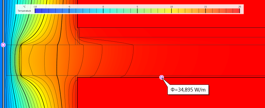
The measurement tool is now setup to sum up all heat fluxes entering the boundary condition external climate inside the rectangular area “Total D” that actually covers our whole simulation. Re-run the thermal simulation using the button T stable solution. After the simulation has finished a new magenta coloured marker will appear. Double-click on it to show the measurement result inside a tag. If you have used the materials and dimensions given in this tutorial and run the simulation with the suggested resolution of 1.5mm the total heat flux should match the value shown below.
To calculate the PSI value based on this total heat flux we will have to use the formula which defines the PSI value:
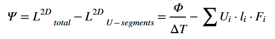
L2D is the heat flux per 1K temperature difference, so you will have to divide the heat flux by the actual temperature difference. From this value you will have to subtract all the “U segments” as they are described in your energy model, using the appropriate U values and lengths. The factor F is a correction factor that is important if you have U sections to warmer areas than the external temperature (like a garage or basement). In our case we have just two external walls included, therefore F will always be 1.0.
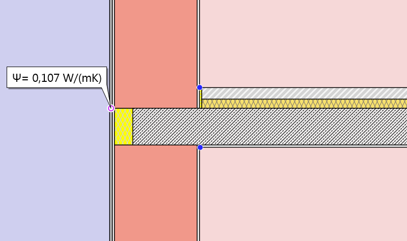
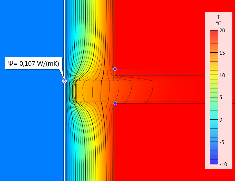
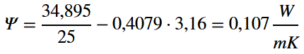
Let’s do the calculation for this example. The heat flux is 34,895 W, the temperature delta is 25 K. The U-value of our wall is 0.4079 W/m²K. Since our upper and lower walls are identical we can just subtract one segment having a total length of 3,16m. So finally we will get:
In accordance with the value that we have determined using the automatic function.
9. Determining the minimum surface temperature and the temperature factor fRSI
Besides calculating the energy loss of a thermal bridging detail (according to ISO 10211) it is often required to proof that the minimum surface temperature in the area of the thermal bridge will stay above certain levels (e.g. mold or dew point temperatures). Once again HTflux offers an automatic tool that will find the positon and temperature of the coldest spot and will also calculate the so-called temperature factor as well as the mold or dew point temperatures.
In central Europe as well as in some other countries it is necessary to this calculation with an altered internal heat film resistance of 0,25 m²K/W. This should reflect a “worst-case” scenario e.g. in corners or when a curtain is covering the wall. This will restrict radiation as well as convection warming of the wall resulting in a higher heat film resistance. If you have you want to use the standard boundary condition you could skip this step, however the task of this tutorial is to make you familiar with HTflux, therefore we will now explain how to create a new boundary condition. To get this new boundary condition we could either change the heat transfer resistance of the existing “internal climate” or we could add a new boundary condition. We will do the latter to get familiar with creating boundary conditions. Right click on an existing “internal climate” boundary condition in the material list on the right side of the screen and select Duplicate.
Double click on then newly create boundary condition to open then boundary dialog. To adjust the b.c. as needed proceed as follows:
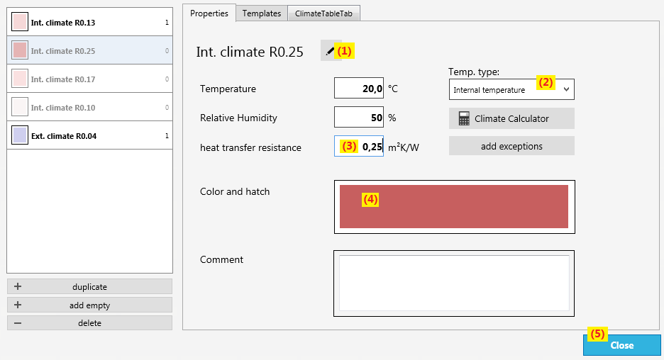
- Click on the pen and enter a new name such as “internal climate R0.25”.
- Make sure the new boundary condition is of type “internal temp”
- Type in the new heat transfer resistance 0.25.
- Double-click on the colour preview and select an appropriate colour (maybe dark red)
- Close the dialog
Now don’t forget to change the assignment with the newly create boundary condition. E.g. by dragging the new “0.25 boundary condition” over the existing one.
Important note: if you are doing the minimum temperature calculation with this boundary condition having a reduced heat transfer (higher resistance value), the result measured by the PSI-tool will not show the correct value, as this calculation will require the standard heat transfers. For this reason you should turn off the result display of the psi-tool. You can either do this by clicking on the eye symbol right to the PSI-tool item in the project manager or by double-clicking on the PSI-marker to only hide the result tag of the tool.
Since this tutorial is designed to train you on HTflux will do another extra job here. We will not only calculate the minimum temperature for the whole simulation, but for each floor individually. Therefore you can click twice on the Surface Temp. button in the Measurements menu:

Two newly created items called “Surf.Temp.1” and “Surf.Temp.2.” will show up in the project manager on the right. To assign different regions to them we will now have to draw two separate regions (instead of duplicating the region “total” as above). To create this two regions simply use the button Region in the Drawing menu:
![]()
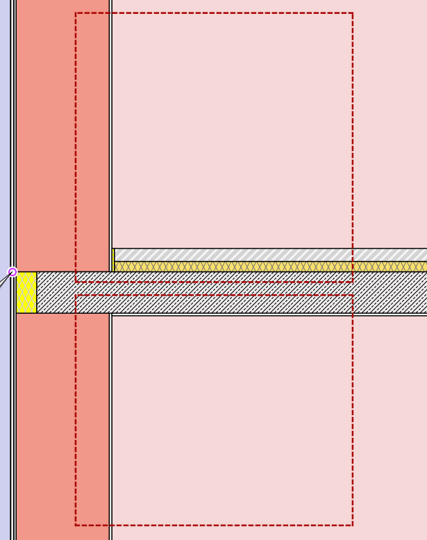
Use the mouse to define two rectangular areas covering the floor and wall area on the top floor and the ceiling and wall area on the bottom floor:
Note: if you have done something wrong you can delete the wrong items with the right click menu in the project manager. The objects draw last will always be the ones on top of the list.
Just like before when working with the heat-flux tool before you can now use mouse dragging (holding the left button down) to assign the two regions to the two surface temperature tools (1)(2):
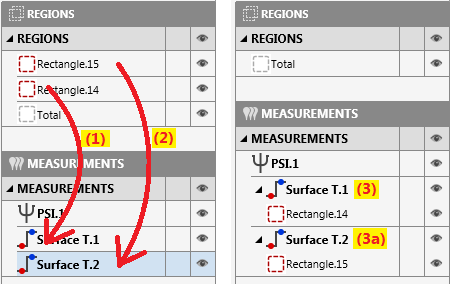
Also very similar to the heat-flux setup double click on the item “Surf.Temp.1” to bring up the setup dialog for this tool. Again, select all materials on the left using the button all (1) on the right list select all the internal climates (2). It would be sufficient to select only the newly create climate “R0.25”, however if you want to change the boundary condition assignment later on, you can make sure it will still work, when having all internal climates selected. Close the dialog (3) and repeat the same process for the other tool called Surf.Temp.2.

Now re-run the simulation using the button T stable solution. Two new markers with blue color and two markers having red color will appear in the simulation. These mark the spots having the lowest and highest temperatures inside the specific regions. We are interested in the minimum temperatures marked by the blue circles. You can also double-click on them to hide or show the results with a tag. Make sure the tags for the blue markers are visible, place them appropriately by dragging with the mouse and double-click inside them to get into the measurement setup dialog.
The measurement dialog for the Surface Temp. tool will come up again, but this time the tab condensation & mold temperatures will be visible. Here you can decide what additional information should be displayed along with the minimum temperature. To show all possible parameters it will be necessary to decide on two reference climates. HTflux will use these temperatures and humidity-values to calculate the temperature factors as well as the mold and dew point temperatures. Selecting an internal reference climate is necessary to calculate the mold and dew point temperature, selecting an external reference climate will allow HTflux to calculate the temperature factore fRsi,min. If you are not interested in these additional information you can skip this step.

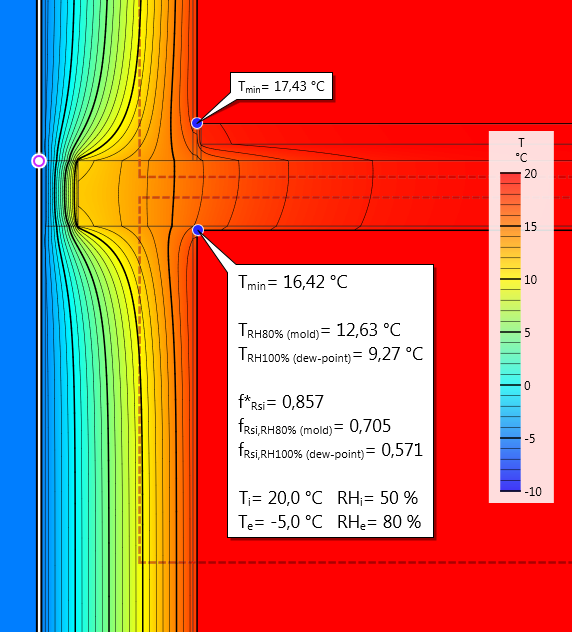
Repeat the process for the other minimum temperature. In our example the lowest temperature will of course be found in the ceiling area of the bottom floor, as the insulation of the floor layers will raise the temperatures on the top floor.
Here we can determine a value of 16,4°C as the lowest temperature. This temperature is above the the mold and dew-point temperature, therefore the thermal bridge will not cause any health risk. The temperature factor is another way of describing this. It relates the temperature difference between the minimum temperature and the external temperature to the total temperature difference:
E.g. according to the German standard DIN 4108 it is obligatory that this value has to be higher than 0.7. This criterion is also met in our example.
Now that we have done all the necessary calculations on the thermal bridge you can use the features of the Image export or PDF-Export tools to do the reporting for this detail.
Here are some examples for possible output formats: